Yes, I realize that after reading the title of this post, 99% of potential readers just kept scrolling. So to the few of you who clicked on it, welcome! Don’t worry, this won’t take long.
A very long time ago, I was curious how to detect the strength of the bass and treble in music, in order to synchronize some graphical effects. I had no idea how to do such a thing, so I tried to figure it out, but I didn’t get very far. Eventually I learned that I needed something called a Fourier transform, so I took a trip to the library and looked it up (which is what we had to do back in those days).
What I found was the Discrete Fourier Transform (DFT), which looks like this:
This formula, as anyone can see, makes no sense at all. I decided that Fourier must have been speaking to aliens, because if you gave me all the time and paper in the world, I would not have been able to come up with that.
Eventually, I was able to visualize how it works, which was a bit of a lightbulb for me. That’s what I want to write about today: an intuitive way to picture the Fourier transform. This may be obvious to you, but it wasn’t to me, so if you work with audio or rendering, I hope there’s something here you find useful.
Disclaimer: my math skills are pitch-patch at best, and this is just intended to be an informal article, so please don’t expect a rigorous treatment. However, I will do my best not to flat-out lie about anything, and I’m sure people will set me straight if I get something wrong.
A quick bit of background – what does the Fourier transform do? It translates between two different ways to represent a signal:
- The time domain representation (a series of evenly spaced samples over time)
- The frequency domain representation (the strength and phase of waves, at different frequencies, that can be used to reconstruct the signal)
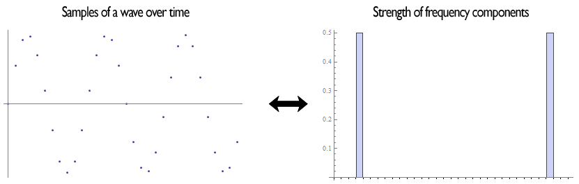
The picture on the left shows 3 cycles of a sine wave, and the picture on the right shows the Fourier transform of those samples. The output bars show energy at 3 cycles (and, confusingly enough, negative 3 cycles… more on that below).
The inputs and outputs are actually complex numbers, so to feed a real signal (like some music) into the Fourier transform, we just set all the imaginary components to zero. And to check the strength of the frequency information, we just look at the magnitude of the outputs, and ignore the phase. But let’s never mind all that for now.
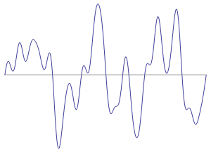
What are we trying to accomplish? We’ve got a sampled signal, and we want to extract frequency information from it. The Fourier transform works on a periodic, or looping signal. This seems like a problem, since we don’t actually have any signals like that. In practice, you just take a small slice of a longer signal, fade both ends to zero so that they can be joined (which is a whole topic unto itself), and pretend it’s a loop.
Let’s make things simple and say that our loop repeats once per second.
Picture it as a bead, sliding up and down along a thin rod, tracing out the signal. So as this bead is bobbing up and down, look what happens if we spin the rod at a rate of, say, 10 revolutions per second:

We get a scribble, as you’d expect. And it is roughly centered on the origin.
Now, let’s assume we know there’s some energy in the signal at 3 Hz, and we want to measure it. What that means is that on top of whatever else is causing the signal to wobble around, we’ve added a wave that oscillates 3 times per second. It has a high point every 1/3 of a second, and corresponding low points in between, also spaced 1/3 of a second apart. You can probably see now how we might be able to detect it… let’s try spinning our signal at a matching rate of 3 revolutions per second.
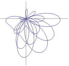
Since the signal completes a rotation every 1/3 of a second, all the high points in our 3 Hz wave line up at the same part of the rotation, and this pulls the whole scribble off-center. How can we quantify that? The easiest way would be to record a bunch of points as we rotate, and average them to find their midpoint:

It makes sense that the distance of this midpoint from the origin is proportional to the strength of the signal, because as the high points in our signal get higher, they will move the scribble farther away. But what if the signal contains no energy at 3 Hz? Let’s remove the 3 Hz wave and see:
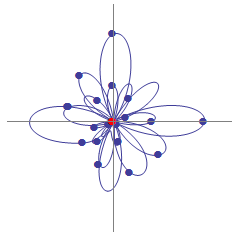
Now there is nothing to pull the scribble off center, and all of the other oscillations tend to (approximately) balance each other out.
This looks promising as a way to detect energy at a given frequency. Time to translate it into math! For a looping signal of N samples:
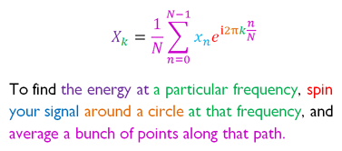
(Raising e to an imaginary power produces rotation around a unit circle in the complex plane, according to Euler’s formula. How? Magic, as far as I can tell. But apparently it’s true).
So this equation is a little different from what we started with. I’ve added a normalization factor of 1/N, and changed the sign of the exponent. I also rearranged the terms slightly for clarity. This form is normally called the inverse DFT, which is confusing, but apparently the difference between the DFT and IDFT is a matter of convention, and can depend on the application. So, let’s call that close enough.

Anyway, once you can “see” what’s going on in your head, a lot of the quirks of working with the DFT become much less mysterious. If you’ve had to work with DFT output before, you may have wondered:
- Why does the first element in the result (k=0) contain the DC offset? Because in that case, our samples don’t spin at all, so all we’re doing is averaging them.
- Why doesn’t the DC offset affect the frequency information? Because adding a constant value to all the samples just makes the whole scribble bigger, which doesn’t affect the midpoint.
- Why does the second half of the output array contain a mirror image of the first half? It’s just our old friend aliasing. When calculating the last element (k=N-1), we’re rotating by (N-1)/N at each step, which is almost all of the way around. This is the same as taking small steps (1/N) in the wrong direction. That’s why the result at (k=N-1) has the same magnitude as (k=1). It’s equivalent to processing a negative frequency of (k=-1).
- Why does a sine wave with amplitude 1.0 come out of the DFT as 0.5? When we spin the sine wave, we get a circle of diameter 1.0, but it’s midpoint is only half that distance away from the origin.
- Where is the other half of the energy then? It’s hiding in the negative frequency part!
Hopefully this was more helpful than confusing.
And if you’d like to get updates on my game development work, come subscribe to my RSS feed at pureenergygames.com!